1. Introduction
This is my first run at a Kaggle competition. I have chosen to tackle the beginner's Titanic survival prediction. I have used as inspiration the kernel of Megan Risdal, and i have built upon it. I will be doing some feature engineering and a lot of illustrative data visualizations along the way. I’ll then use randomForest to create a model predicting survival on the Titanic. I am new to machine learning and data science and i hope to learn a lot from these datasets! There are three parts to my script as follows:
- Feature engineering
- Missing value imputation
- Prediction!
1.1 Load libraries and check the data
library('ggplot2') # visualization
library('ggthemes') # visualization
library('scales') # visualization
library('dplyr') # data manipulation
library('mice') # imputation
library('randomForest') # classification algorithm
library('plyr') # feature correlation
library('corrplot') # feature correlation plotting
Now that the packages are added, we will add the relevant tables with train, test and ethnicity data.
testDat <- read.csv("../input/titanic/test.csv",stringsAsFactors = F)
trainDat <- read.csv("../input/titanic/train.csv",stringsAsFactors = F)
totalDat <- bind_rows(trainDat, testDat) # bind training & test data
ethnicityDat <- read.csv("../input/ethnicity/ethnicity.csv", stringsAsFactors = F)
Let's have a look at the data.
str(totalDat) # check full data'data.frame': 1309 obs. of 12 variables:
$ PassengerId: int 1 2 3 4 5 6 7 8 9 10 ...
$ Survived : int 0 1 1 1 0 0 0 0 1 1 ...
$ Pclass : int 3 1 3 1 3 3 1 3 3 2 ...
$ Name : chr "Braund, Mr. Owen Harris" "Cumings, Mrs. John Bradley (Florence Briggs Thayer)" "Heikkinen, Miss. Laina" "Futrelle, Mrs. Jacques Heath (Lily May Peel)" ...
$ Sex : chr "male" "female" "female" "female" ...
$ Age : num 22 38 26 35 35 NA 54 2 27 14 ...
$ SibSp : int 1 1 0 1 0 0 0 3 0 1 ...
$ Parch : int 0 0 0 0 0 0 0 1 2 0 ...
$ Ticket : chr "A/5 21171" "PC 17599" "STON/O2. 3101282" "113803" ...
$ Fare : num 7.25 71.28 7.92 53.1 8.05 ...
$ Cabin : chr "" "C85" "" "C123" ...
$ Embarked : chr "S" "C" "S" "S" ...str(ethnicityDat) # check ethnicity data'data.frame': 1630 obs. of 2 variables:
$ Name: chr "april" "june" "august" "jun" ...
$ Eth : chr "HISPANIC" "WHITE NON HISPANIC" "WHITE NON HISPANIC" "ASIAN AND PACIFIC ISLANDER" ...We’ve got a sense of our variables, their class type, and the first few observations of each. We know we’re working with 1309 observations of 12 variables and 1630 observations of 2 variables. To make things a bit more explicit since a couple of the variable names aren’t 100% illuminating, here’s what we’ve got to deal with:
| totalDat |
|---|
| Name | Description |
|---|---|
| PassengerId | The unique passenger Id |
| Survived | Survived [1] or died [0] |
| Pclass | Passenger's class [1,2,3] |
| Name | Passenger's names and title |
| Sex | Passenger's sex |
| Age | Passenger's age |
| SibSp | Number of siblings/spouses aboard |
| Parch | Number of parents/children aboard |
| Ticket | Ticket number |
| Fare | Ticket price |
| Cabin | Cabin number |
| Embarked | Port of embarkment |
| ethnicityDat |
|---|
| Name | Description |
|---|---|
| Name | First name |
| Eth | Ethnicity based on the name given |
2. Feature Engineering
The second step is the most important step! Even though we have a lot of features already, we would need to impute the missing values and also look for correlations and features that could have influenced the passenger's survival.
2.1 What's in a name?
The first variable which i would work on is the passenger's name because we can break it down into additional meaningful variables which can feed predictions or be used in the creation of additional new features. For instance, passenger title is contained within the passenger name variable, we can use surname to represent families, we can use given name to match it with the ethnicity of the passenger.
totalDat$Title <- gsub('(.*, )|(\\..*)', '', totalDat$Name) # Extract the title from the name
totalDat$Surname <- tolower(sapply(totalDat$Name,function(x) {strsplit(x, split = '[,.]')[[1]][1]})) # Extract the Surname
Name <- sapply(totalDat$Name, function(x) {strsplit(x, split='[,.]')[[1]][3]})
Names <- sapply(Name, function(x) {strsplit(x, split=' ')[[1]][2]}) # Extract the given Name
mat  <- matrix(unlist(Names), ncol=1, byrow=TRUE)
mat <- gsub("[[:punct:]]","",mat)
totalDat$Given<- tolower(mat)
totalDat$Given <- totalDat$Given[,]
totalDat <- merge(totalDat,ethnicityDat,by.x="Given",by.y="Name",all.x=T) # Merge with ethnicityDat
colnames(totalDat)[colnames(totalDat)=='Eth'] <- 'Ethnicity' # Rename Eth to Ethnicity
Let's have a look at the Titles distributions for each of the sexes
table(totalDat$Sex, totalDat$Title) # create a table which shows all of the title combinations Capt Col Don Dona Dr Jonkheer Lady Major Master Miss Mlle Mme Mr Mrs
female 0 0 0 1 1 0 1 0 0 260 2 1 0 197
male 1 4 1 0 7 1 0 2 61 0 0 0 757 0
Ms Rev Sir the Countess
female 2 0 0 1
male 0 8 1 0There are titles with a very low amount of people sharing them. We will aggregate the rare titles in their own sub-groups.
officer_title <- c('Capt','Col','Major')
community_title <- c('Dr','Sir')
rare_title <- c('Dona', 'Lady', 'the Countess', 'Don', 'Rev', 'Jonkheer')
totalDat$Title[totalDat$Title == 'Mlle']        <- 'Miss'
totalDat$Title[totalDat$Title == 'Ms']          <- 'Miss'
totalDat$Title[totalDat$Title == 'Mme']         <- 'Mrs'
totalDat$Title[totalDat$Title %in% rare_title]  <- 'Rare Title'
totalDat$Title[totalDat$Title %in% officer_title]  <- 'Crew'
totalDat$Title[totalDat$Title %in% community_title]  <- 'Member'
Thus the list of titles now looks more generalized.
table(totalDat$Sex,totalDat$Title) Crew Master Member Miss Mr Mrs Rare Title
female 0 0 1 264 0 198 3
male 7 61 8 0 757 0 102.2 Will larger families deal better with the crash?
Now that we’ve taken care of splitting passenger name into some new variables, we can take it a step further and make some new family variables. First we’re going to make a family size variable based on number of siblings/spouse(s) (maybe someone has more than one spouse?) and number of children/parents.
Let's aggregate the family sizes and check their survival rates.
totalDat$Fsize <- totalDat$SibSp + totalDat$Parch + 1 # Passenger + Siblings/Spouses + Parents/Children
totalDat$IsAlone[totalDat$Fsize==1] <- 'Alone' # Is the passenger travelling alone?
totalDat$IsAlone[totalDat$Fsize!=1] <- 'Not Alone'
totalDat$IsAlone <- factor(totalDat$IsAlone)
totalDat$Family <- paste(totalDat$Surname, totalDat$Fsize, sep='_') # families Surname
Let's have a look at the survival rates now.
totalDat <- totalDat[order(totalDat$PassengerId),] #Sort the data
ggplot(totalDat[1:891,], aes(x = Fsize, fill = factor(Survived))) +
  geom_bar(stat='bin', position='dodge') +
  scale_x_continuous(breaks=c(1:11)) +
  labs(x = 'Family Size') +
  theme_few()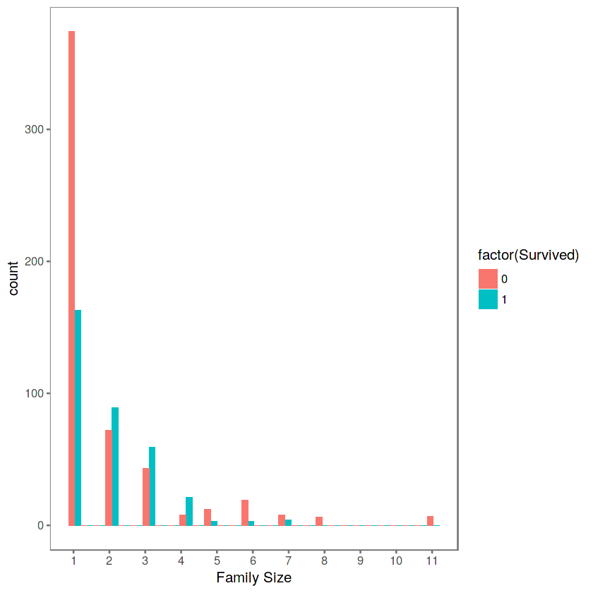
We can see that there’s a survival penalty to singletons and those with family sizes above 4. We can collapse this variable into three levels which will be helpful since there are comparatively fewer large families. Let’s create a discretized family size variable.
totalDat$FsizeD[totalDat$Fsize == 1] <- 'singleton'
totalDat$FsizeD[totalDat$Fsize < 5 & totalDat$Fsize > 1] <- 'small'
totalDat$FsizeD[totalDat$Fsize > 4] <- 'large'
mosaicplot(table(totalDat$FsizeD, totalDat$Survived), main='Family Size by Survival', shade=TRUE) # Plotting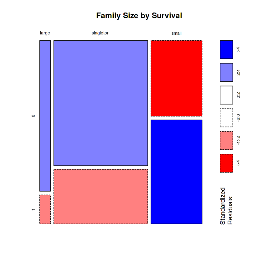
The mosaic plot shows that we preserve our rule that there’s a survival penalty among singletons and large families, but a benefit for passengers in small families. I want to do something further with our age variable, but 263 rows have missing age values, so we will have to wait until after we address missingness.
2.3 Travelling with your friends?
An interesting detail is that there are duplicate tickets. This infers that people travelled together without the need of being relatives. These tickets also share identical fares, which implies that the ticket fare should be divided by the number of people buying it. This will give us a better overview of ticket prices based on different features.
n_occur <- data.frame(table(totalDat$Ticket))
totalDat <- merge(totalDat,n_occur, by.x="Ticket", by.y="Var1", x.all=T) # Assign the frequency of each ticket appearance
totalDat$Fare <- totalDat$Fare / totalDat$Freq # Recalculate the fares accordingly
2.4 What are these letters in the Cabin column?
The Cabin values indicate that there are three parameters. The first one is always a letter. Each letter corresponds to the deck in which the room could be found. We must investigate if being located on a given deck would increase your chances of survival.
totalDat$Deck<-factor(sapply(totalDat$Cabin, function(x) {strsplit(x, NULL)[[1]][1]}))Let's have a look at the Deck/Survived distributions
totalDat <- totalDat[order(totalDat$PassengerId),]
totalDat$Deck[totalDat$Deck=='']<-NA
totalDat$Deck <- factor(totalDat$Deck)
totalDat$Deck <- addNA(totalDat$Deck)
ggplot(totalDat[1:891,],aes(x=Deck,fill=factor(Survived)))+geom_bar()+scale_fill_discrete("Survived?")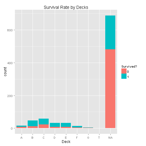
Looks like there are alot of missing values. Let's look at the data without these missing values.
levels(totalDat$Deck)[9] <- "TT"
train <- totalDat[1:891,] # Look only at Data with known survival
ggplot(train[train$Deck!='TT',],aes(x=Deck,fill=factor(Survived)))+geom_bar()+scale_fill_discrete("Survived?")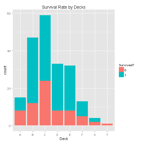
There seems to be some correlation, but with so much missing values it would not make sense to draw conclusions.
3 Missing values
Before we continue with the feature engineering, we must handle missing values. There are missing values in the Age, Fare, Embarked and Deck
3.1 Embarked and Fare missing values
When we check for missing values in the Fare column we find that row 1044 has a missing Fare. This is a passenger from third class, which embarked from port S. We will give him a Fare which corresponds to the median Fare for this case.
totalDat$Fare[1044] <- median(totalDat[totalDat$Pclass == '3' & totalDat$Embarked == 'S', ]$Fare, na.rm = TRUE)Looking at Embarked, the rows with number 62 and 830 don't have a value for Embarked. Let's look at how much these passengers paid for their tickets and where would they be placed according to their class and fare
totalDat$Fare[totalDat$PassengerId==62][1]
totalDat$Fare[totalDat$PassengerId==830][1]
40
40Aha! It seems that both passengers paid the same amount - 40$. Let's check where this lands compared with the median fare for each port.
embark_fare <- totalDat %>% filter(PassengerId != 62 & PassengerId != 830)
ggplot(embark_fare, aes(x = Embarked, y = Fare, fill = factor(Pclass))) +
  geom_boxplot() +
  geom_hline(aes(yintercept=40), colour='red', linetype='dashed', lwd=2) +
  scale_y_continuous(labels=dollar_format()) +
  scale_fill_discrete("Passenger class") +
  labs(title= "Fares by Embarked") +
  theme_few()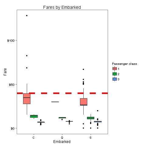
The fare which these passengers paid is closest to the median of 1st class in port C
totalDat$Embarked[c(62, 830)] <- 'C'3.2 Imputation of missing values in Age
So, there are quite a few missing Age values in our data. We are going to get a bit more fancy in imputing missing age values. Why? Because we can. We will create a model predicting ages based on other variables. Let's have a look at how many values need imputation.
sum(is.na(totalDat$Age))263The first step would be to factor the variables and then use mice to predict the Age.
totalDat$PassengerId <- factor(totalDat$PassengerId)
totalDat$Pclass <- factor(totalDat$Pclass)
totalDat$Sex <- factor(totalDat$Sex)
totalDat$Embarked <- factor(totalDat$Embarked)
totalDat$Title <- factor(totalDat$Title)
totalDat$Surname <- factor(totalDat$Surname)
totalDat$Family <- factor(totalDat$Family)
totalDat$FsizeD <- factor(totalDat$FsizeD)
totalDat$Ethnicity <- factor(totalDat$Ethnicity)
set.seed(129)
mice_mod <- mice(totalDat[, !names(totalDat) %in% c('PassengerId','Name','Ticket',
			'Cabin','Family','Surname','Survived','Ethnicity')], method='rf')
mice_output <- complete(mice_mod)
iter imp variable
1 1 Age
1 2 Age
1 3 Age
1 4 Age
1 5 Age
2 1 Age
2 2 Age
2 3 Age
2 4 Age
2 5 Age
3 1 Age
3 2 Age
3 3 Age
3 4 Age
3 5 Age
4 1 Age
4 2 Age
4 3 Age
4 4 Age
4 5 Age
5 1 Age
5 2 Age
5 3 Age
5 4 Age
5 5 AgeLet's have a look if the imputed age follows the pattern of the existing model.
par(mfrow=c(1,2))
hist(totalDat$Age, freq=F, main='Age: Original Data',
  col='darkgreen', ylim=c(0,0.04))
hist(mice_output$Age, freq=F, main='Age: MICE Output',
  col='lightgreen', ylim=c(0,0.04))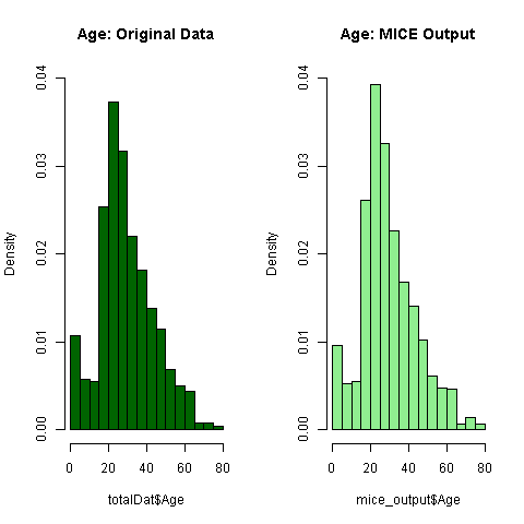
Everything seems to look normal, thus let's assign the imputed values to the missing ones.
totalDat$Age <- mice_output$Age3.3 Feature Engineering round 2
Now that we know everyone’s age, we can create a couple of new age-dependent variables: Child and Mother. A child will simply be someone under 18 years of age and a mother is a passenger who is 1) female, 2) is over 18, 3) has more than 0 children (no kidding!), and 4) does not have the title ‘Miss’. First off let's see if there is a relationship between Age, Survived and Sex.
ggplot(totalDat[1:891,], aes(Age, fill = factor(Survived))) +
  geom_histogram() +
  # I include Sex since we know (a priori) it's a significant predictor
  # "Women and children first!"
  facet_grid(.~Sex) +
  theme_few()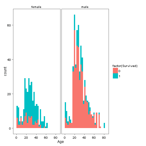
So it looks like if you are a Woman or a Child you have higher chances of survival, not so large but still larger than being a male. Lets create the new groups Child and Mother.
totalDat$Child[totalDat$Age < 18] <- 'Child'
totalDat$Child[totalDat$Age >= 18] <- 'Adult'
totalDat$Mother <- 'Not Mother'
totalDat$Mother[totalDat$Sex == 'female' & totalDat$Parch > 0 & totalDat$Age > 18 & totalDat$Title != 'Miss'] <- 'Mother'
totalDat$Child  <- factor(totalDat$Child)
totalDat$Mother <- factor(totalDat$Mother)
So here is where Megan Risdal decided to stop and i will contribute with my findings.
4 Feature Engineering round 3
I will be further investigating the Deck missing values. Is there any relation between which class you are in and your Sex, Age or Ethnicity?
4.1 Is ethnicity a factor for your survival aboard the Titanic?
By using the Ethnicity dataset we have added the most common ethnicity in relation to the passenger's Name. Is there any relation between which class you are in and your Sex, Age or Ethnicity? Let's have a look at the ethnicity data.
levels(totalDat$Ethnicity)''
'Asian And Pacific Islander'
'Black Non Hispanic'
'Hispanic'
'White Non Hispanic'#Let's replace the values with shorter and more clear versions
totalDat$Ethnicity <- addNA(totalDat$Ethnicity)
levels(totalDat$Ethnicity)[is.na(levels(totalDat$Ethnicity))] <- 'NaN'
levels(totalDat$Ethnicity)[tolower(levels(totalDat$Ethnicity))=='asian and pacific islander'] <- 'Asian'
levels(totalDat$Ethnicity)[tolower(levels(totalDat$Ethnicity))=='black non hispanic'] <- 'Black'
levels(totalDat$Ethnicity)[tolower(levels(totalDat$Ethnicity))=='white non hispanic'] <- 'White'
levels(totalDat$Ethnicity)[tolower(levels(totalDat$Ethnicity))=='hispanic'] <- 'Hispanic'
totalDat <- totalDat[order(totalDat$PassengerId),]
levels(totalDat$Ethnicity) #And the new levels are 'NaN'
'Asian'
'Black'
'Hispanic'
'White'ggplot(totalDat[1:891,],aes(x=Ethnicity,fill=factor(Survived))) +
geom_bar() +
scale_fill_discrete("Survived?") +
labs(title= "Survival Rate by Ethnicity")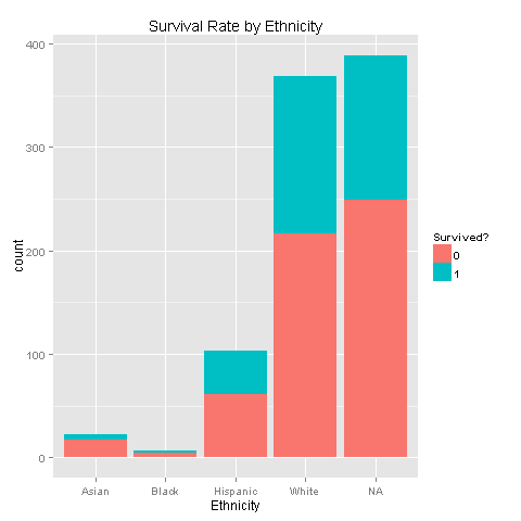
One could easily see that each of the ethnic groups has the exact same survival chances. Another thing to notice is that most of the passengers were White, and even if we imputed Ethnicity we would not achieve good results but just increase noise. Nevertheless, let's dig deeper and look for Ethnicity, Survived and Sex relations.
ggplot(totalDat[1:891,],aes(x=Ethnicity,fill=factor(Survived))) +
 		geom_bar() +
 		scale_fill_discrete("Survived?") +
labs(title= "Survival Rate by Ethnicity") +
facet_grid(.~Sex)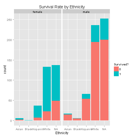
Still nothing. Females get to survive more, without any ethnicity boost. Carry on, there must something else.
4.2 Is Class a significant factor for your survival?
When i watched the movie i felt like 1st and 2nd class were placed on higher decks than 3rd class. I guess we need to investigate that.
ggplot(totalDat[totalDat$Deck!='TT',],aes(x=factor(Deck),fill=factor(Pclass))) +
 		geom_bar() +
 		scale_fill_discrete("Class") +
 		labs(title= "Class separation by decks",x = 'Deck')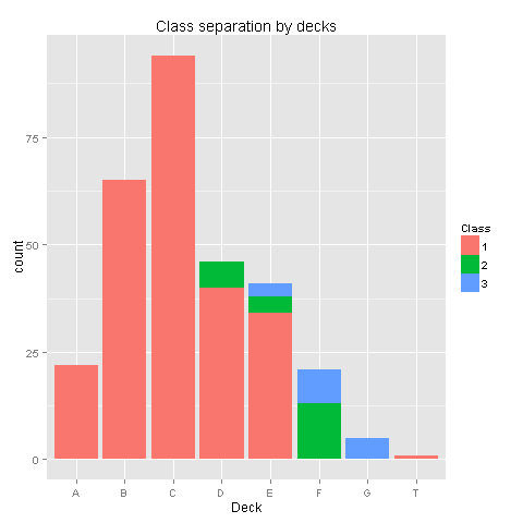
Yes, there is a pattern here! Class 1 was placed on decks A to E, Class 2 was placed on decks D,E,F and Class 3 was placed on decks E,F,G. Deck T was habitated by a small group from Class 1. Even though we have found a pattern, the amount of missing values in the Deck column would make any assumptions easy to reject. Nevertheless we know for sure that people from class 3 were at the lower parts of the ship. Let's check if your survival is somewhat dependent on your class and sex.
ggplot(totalDat[1:891,],aes(x=factor(Pclass),fill=factor(Survived))) +
 		geom_bar() +
 		scale_fill_discrete("Survived?") +
 		labs(title= "Class survival by sex",x = 'Class') +
        facet_grid(.~Sex)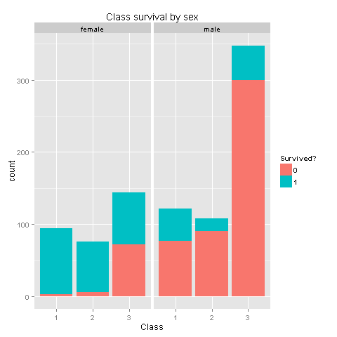
Wow! We knew that women had higher chances of survival, but women from Class 3 don't have high survival rates. I wonder if this has something to do with being placed at the lower levels of the ship. If women from class 3 were not having high odds, could we state the same for children from class 3?
ggplot(totalDat[1:891,],aes(x=factor(Pclass),fill=factor(Survived))) +
 		geom_bar() +
 		scale_fill_discrete("Survived?") +
 		labs(title= "Child survival by class",x = 'Class') +
		facet_grid(.~Child)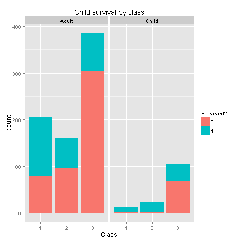
Well, well, well. I believe we have found gold here. From the last 2 graphs one could easily see that if you were a woman, or a child from classes 1 and 2 you had really high chances of survival! Women or children from class 3 had survival chances equal to those of men. Let's create new features based on our findings.
totalDat$ChildFrom12 <- 'Not from'
totalDat$ChildFrom12[totalDat$Child=='Child'&totalDat$Pclass==1] <- 'From'
totalDat$ChildFrom12[totalDat$Child=='Child'&totalDat$Pclass==2] <- 'From'
totalDat$ChildFrom12 <- factor(totalDat$ChildFrom12)
totalDat$FemaleFrom12 <- 'Not from'
totalDat$FemaleFrom12[totalDat$Sex=='female'&totalDat$Pclass==1] <- 'From'
totalDat$FemaleFrom12[totalDat$Sex=='female'&totalDat$Pclass==2] <- 'From'
totalDat$FemaleFrom12 <- factor(totalDat$FemaleFrom12)
Probably we will find the same class survival for women that are Mothers or not.
ggplot(totalDat[1:891,],aes(x=Mother,fill=factor(Survived))) +
 		geom_bar() +
 		scale_fill_discrete("Survived?") +
 		labs(title= "Survival of Mother by Class",x = 'Mother') +
        	facet_grid(.~Pclass)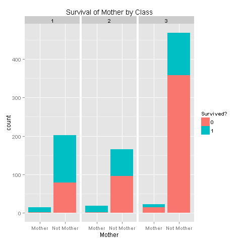
So there's a strong relation with survival depending on your class. It would be awesome if we could have had more Deck values in order to further be able to state that people on the lower decks had bad luck. Let's add this new feature to our data.frame.
totalDat$MotherFrom12 <- 'Not from'
totalDat$MotherFrom12[totalDat$Mother=='Mother'&totalDat$Pclass==1] <- 'From'
totalDat$MotherFrom12[totalDat$Mother=='Mother'&totalDat$Pclass==2] <- 'From'
totalDat$MotherFrom12 <- factor(totalDat$MotherFrom12)
4.3 Is there a family size and child relation?
Lets check if there are relations between family size, child and sex.
ggplot(totalDat[1:891,],aes(x=factor(Child),fill=factor(Survived))) +
 		geom_bar() +
 		scale_fill_discrete("Survived?") +
 		labs(title= "Survival by Child, Discrete family Size and Sex",x = 'Child') +
		facet_grid(.~FsizeD+Sex)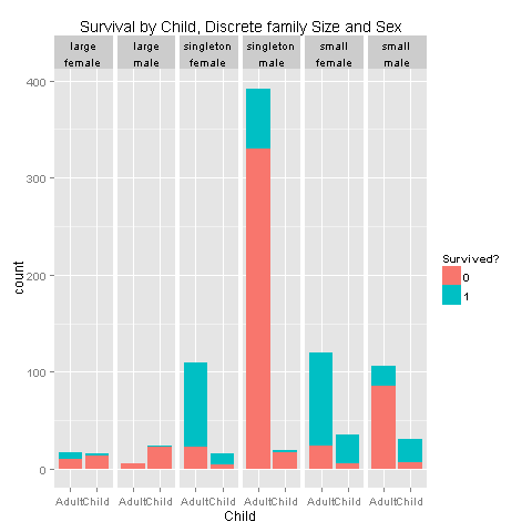
I would say that i see a pattern for children from small families, and singletons. Let's create a feature that describes those relationships.
totalDat$ChildSaved <- 'Not saved'
totalDat$ChildSaved[totalDat$Child=='Child'&totalDat$Sex=='female'&totalDat$FsizeD!='large'] <- 'Saved'
totalDat$ChildSaved[totalDat$Child=='Child'&totalDat$Sex=='male'&totalDat$FsizeD=='small'] <- 'Saved'
totalDat$ChildSaved <- factor(totalDat$ChildSaved)
4.4 Feature correlation
We will visualize the correlation between features in order to have some insight on the features that are strong enough for our prediction model.
corr_data <- totalDat[1:891,]
## transform to numeric type and recodification
corr_data$Embarked <- revalue(corr_data$Embarked,
			c("S" = 1, "Q" = 2, "C" = 3))
corr_data$Sex <- revalue(corr_data$Sex,
			c("male" = 1, "female" = 2))
corr_data$Title <- revalue(corr_data$Title,
			c("Mr" = 1, "Master" = 2,"Crew" = 3,
			"Mrs" = 4,"Member" = 5,"Miss" = 6, "Rare Title" = 7))
corr_data$FsizeD <- revalue(corr_data$FsizeD,
			c("small" = 1, "singleton" = 2, "large" = 3))
corr_data$Child <- revalue(corr_data$Child,
			c("Adult" = 1, "Child" = 2))
corr_data$Mother <- revalue(corr_data$Mother,
			c("Mother" = 1, "Not Mother" = 2))
corr_data$Mother <- as.numeric(corr_data$Mother)
corr_data$FsizeD <- as.numeric(corr_data$FsizeD)
corr_data$Child <- as.numeric(corr_data$Child)
corr_data$Sex <- as.numeric(corr_data$Sex)
corr_data$Embarked <- as.numeric(corr_data$Embarked)
corr_data$Title <- as.numeric(corr_data$Title)
corr_data$Pclass <- as.numeric(corr_data$Pclass)
corr_data$Survived <- as.numeric(corr_data$Survived)
corr_data$Freq <- as.numeric(corr_data$Freq)
corr_data$Age <- as.numeric(corr_data$Age)
corr_data$ChildFrom12 <- as.numeric(revalue(corr_data$ChildFrom12,
			c("From"=1,"Not from" = 2)))
corr_data$FemaleFrom12 <- as.numeric(revalue(corr_data$FemaleFrom12,
			c("From"=1,"Not from" = 2)))
corr_data$MotherFrom12 <- as.numeric(revalue(corr_data$MotherFrom12,
			c("From"=1,"Not from" = 2)))
corr_data <-corr_data[,c("Survived", "Pclass", "Sex",
			"FsizeD", "Age", "Fare", "Mother",
			"Embarked","Title","Child","ChildFrom12",
			"FemaleFrom12","Freq","MotherFrom12")]
mcorr_data <- cor(corr_data)
corrplot(mcorr_data,method="circle")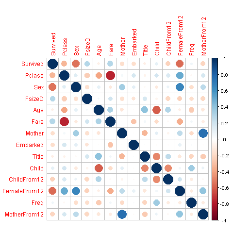
5 Prediction
At last we're ready to predict who survives among passengers of the Titanic based on variables that we carefully curated and treated for missing values. For this, we will rely on the randomForest classification algorithm.
5.1 Bulding the model
The first task on our to-do list is to separate the original file into training and test data.
# Split the data back into a train set and a test set
train <- totalDat[1:891,]
test <- totalDat[892:1309,]
We then build our model using randomForest on the training set. I will not be using Age, Deck or Ethnicity because of the amount of missing values. Imputing does cause noise. The chosen parameters work great and achieve 83.6% model accuracy.
set.seed(156)
rf_model <- randomForest(factor(Survived) ~ Pclass + Sex + Fare + Embarked + Title +
			FsizeD + Freq + ChildSaved + FemaleFrom12 + ChildFrom12, data = train, trees=500)
plot(rf_model, ylim=c(0,0.36))
legend('topright', colnames(rf_model$err.rate), col=1:3, fill=1:3)
rf.fitted = predict(rf_model)
ans_rf = rep(NA,891)
for(i in 1:891){
  ans_rf[i] = as.integer(rf.fitted[[i]]) - 1
}
# Result
table(ans_rf)

print(rf_model)
mean(ans_rf == train$Survived)
varImpPlot(rf_model, main = "RF_MODEL")
# Var importancies
importance    <- importance(rf_model)
varImportance <- data.frame(Variables = row.names(importance),
                            Importance = round(importance[ ,'MeanDecreaseGini'],2))

# var imp
rankImportance <- varImportance %>%
  mutate(Rank = paste0('#',dense_rank(desc(Importance))))

# Graph importancies
ggplot(rankImportance, aes(x = reorder(Variables, Importance),
                           y = Importance, fill = Importance)) +
  geom_bar(stat='identity') +
  geom_text(aes(x = Variables, y = 0.5, label = Rank),
            hjust=0, vjust=0.55, size = 4, colour = 'red') +
  labs(x = 'Variables') +
  coord_flip()
ans_rf
  0   1
603 288


Call:
 randomForest(formula = factor(Survived) ~ Pclass + Sex + Fare +      Embarked + Title + FsizeD + Freq + ChildSaved + FemaleFrom12 +      ChildFrom12, data = train, trees = 5000)
               Type of random forest: classification
                     Number of trees: 500
No. of variables tried at each split: 3

        OOB estimate of  error rate: 16.39%
Confusion matrix:
    0   1 class.error
0 503  46  0.08378871
1 100 242  0.29239766

0.836139169472503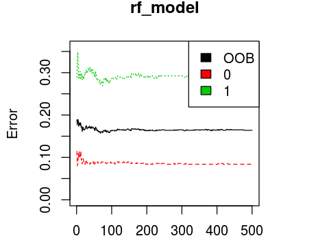
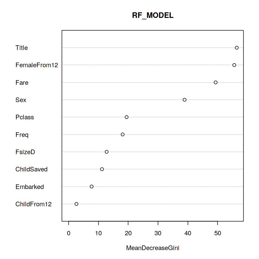
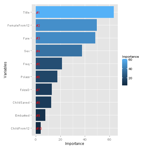
Whoa, glad we made our title variable! It has the highest relative importance out of all of our predictor variables. I think I’m most surprised to see that FemaleFrom12 has such high importance.
5.2 Prediction!
We’re ready for the final step — making our prediction! When we finish here, we could iterate through the preceding steps making tweaks as we go or fit the data using different models or use different combinations of variables to achieve better predictions. But this is a good starting (and stopping) point for me now.
# Predict using the test set
prediction <- predict(rf_model, test)

# Save the solution to a dataframe with two columns: PassengerId and Survived (prediction)
solution <- data.frame(PassengerID = test$PassengerId, Survived = prediction)

# Write the solution to file
write.csv(solution, file = 'rf_mod_Solution.csv', row.names = F)
6 Conclusion
Thank you for taking the time to read through my first exploration of a Kaggle dataset. I look forward to doing more. Again, I would like to thank Megan Risdal for the initial steps of this exploration! The final score i achieved was 0.81818 which is in the top 3% and on 264th place from 8664 competitors.


